How to Freeze Panes in Excel to Lock Rows and Columns (Step-by-Step)

Learning how to freeze panes in Excel is essential when working with large datasets that require scrolling.

This guide shows you exactly how to lock your header rows and columns so they remain visible at all times, ensuring you never lose track of your data labels.

Why Freeze Rows and Columns?

When navigating extensive spreadsheets, scrolling down usually hides your top header row, making it difficult to identify what data belongs to which category. By using the Freeze Panes feature located in the View tab, you “lock” specific areas of the sheet.

This keeps key information static while the rest of the grid scrolls freely, improving data comparison and reducing entry errors.

Below are the three methods to handle this, starting with the most common requirement: locking the top row.

How to Freeze Panes in Excel

Method 1: How to Freeze the Top Row (Quickest Solution)

If your dataset has a single header row at the very top (Row 1) and you want it to stay visible while you scroll down, follow these steps. This is the most frequently used command in the Window group.

1. Open your worksheet and ensure you are in the Normal view.
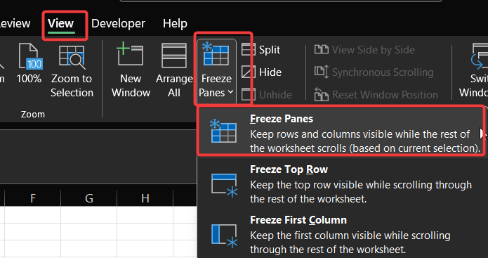
2. Navigate to the View tab on the Excel ribbon.
3. Click on the Freeze Panes dropdown menu.
4. Select Freeze Top Row.

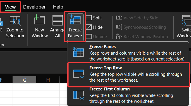
Visual Confirmation: You will see a thin, solid grey line appear underneath Row 1. This indicates the lock is active. Now, when you scroll down to row 100, Row 1 remains fixed at the top.

Method 2: How to Freeze the First Column

If you are working with wide data tables and need to keep names or IDs in Column A visible while scrolling horizontally to the right, use this method.

1. Go to the View tab.
2. Click Freeze Panes.
3. Select Freeze First Column.

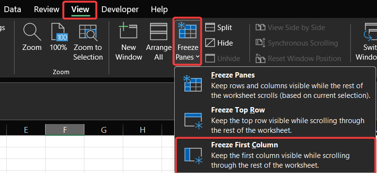
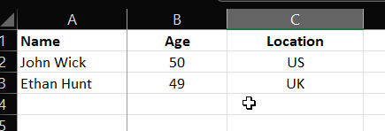
A thin grey line will now appear to the right of Column A, signaling that the specific pane is locked.

Method 3: Freezing Multiple Rows and Columns (The “Magic Cell” Trick)

Do you need to lock more than just the first row or column? Perhaps you need to see the first three rows and the first two columns simultaneously. This requires selecting a specific “anchor cell” before applying the freeze command.

The rule for the anchor cell is simple: Select the cell immediately BELOW the rows and to the RIGHT of the columns you want to freeze.

Step-by-Step Example:

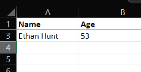
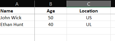
Let’s say you want to freeze Rows 1 and Column A.

1. Identify your anchor cell. Since you want to lock Row 1, you must be below it (Row 2). Since you want to lock Column A, you must be to the right of it (Column B).
2. Click to select cell B3.
3. Go to the View tab and click the Freeze Panes dropdown.
4. Select the first option: Freeze Panes.

Once clicked, Excel divides the window into distinct panes at your selection point. You can now scroll freely in the lower-right section while your headers remain fixed.

Note: Learn more about Microsoft Excel here.

Common Mistakes: Where Should I Click?

When using the “Magic Cell” method, placement is critical. Here is what happens if you click the wrong area:

• Selecting Cell A1: If you select A1 and click Freeze Panes, Excel often defaults to freezing the center of the visible window, creating four arbitrary locked quadrants. This is rarely what you want.
• Selecting a Whole Row: If you select the entire Row 2 (by clicking the number 2 on the left) and click Freeze Panes, Excel will lock only Row 1. It ignores the column selection.
• Selecting a Whole Column: Similarly, selecting the entire Column B will only lock Column A.

Always click a single specific cell to ensure Excel understands exactly where to intersect the freeze lines.

Alternative Method: Using Excel Tables

Did you know you might not need to use Freeze Panes at all? If you are working with a structured dataset, you can format it as an official Excel Table.

1. Select your data range.
2. Press Ctrl + T on your keyboard (or go to Insert > Table).
3. Ensure “My table has headers” is checked.

When you scroll down in an Excel Table, the column letters (A, B, C) are automatically replaced by your actual header names. This is a dynamic alternative to freezing panes that works automatically.

Freeze Panes vs. Split Panes: What’s the Difference?

You may notice a button labeled Split right next to Freeze Panes. While they look similar, they serve different user intents:

• Freeze Panes: Locks rows/columns in place so they cannot move. This is best for headers.
• Split Panes: Divides the window into two or four scrollable areas. Each area can scroll independently. This is best for comparing data from Row 10 with data from Row 500 side-by-side.

To use Split, simply click the Split button in the View tab. To remove it, click Split again.

Advanced Tip: How to Make the Freeze Line Visible

A common user complaint is that the default grey freeze line is too faint, especially on high-resolution monitors. While Microsoft Excel does not allow you to change the color or thickness of the freeze line system-wide, you can use this formatting workaround to make it clearer:

1. Identify the row that is frozen (e.g., Row 1).
2. Highlight the entire row.
3. Go to the Home tab and click the Borders dropdown.
4. Select Thick Bottom Border.

This adds a high-contrast black line exactly where the pane freezes, giving you a clear visual boundary that is easier to see than the default system line.

Pro Tip: The “New Window” Workaround for Dual Monitors

Freeze Panes has one major limitation: it only works within a single window. If you have two monitors and want to view the top of your sheet on Screen 1 and the bottom of your sheet on Screen 2, “Freezing” won’t help.

Instead, use the New Window feature:

1. Go to the View tab.
2. Click New Window.

This opens a second instance of the same workbook. You can keep the header visible on one screen while scrolling to row 10,000 on the other. This is often superior to freezing panes for heavy data analysis.

How to Unfreeze Panes

Knowing how to freeze panes in Excel is only half the battle; you also need to know how to unlock them to return your sheet to normal.

1. Go to the View tab.
2. Click the Freeze Panes dropdown button.
3. Select Unfreeze Panes.

Note: The “Unfreeze” option only appears if panes are currently locked. If nothing is locked, this option will not be visible.

Automation: VBA Macro to Toggle Freeze

For advanced users who toggle this feature constantly, navigating the Ribbon is too slow. You can create a simple macro to toggle the freeze on and off instantly.

1. Press Alt + F11 to open the VBA Editor.
2. Insert a new Module.
3. Paste this code:codeVbaSub ToggleFreezePanes() ActiveWindow.FreezePanes = Not ActiveWindow.FreezePanes End Sub
4. Assign this macro to a button or keyboard shortcut. Now, a single click will lock or unlock your panes instantly based on your current selection.

Platform Specifics: Mac and Mobile Instructions

While the steps above cover Windows, the interface varies slightly on other devices.

For Mac Users:
The process is nearly identical to Windows. Go to the View tab > Freeze Panes. However, if you are using an older version of Excel for Mac without the Ribbon, you may find this option in the top menu bar under Window > Freeze Panes.

For iPhone/Android (Excel Mobile App):

1. Tap on the row or column you want to freeze (or the “Magic Cell” for both).
2. Tap the Ribbon menu (the arrow icon at the bottom right on mobile).
3. Switch from the Home tab to the View tab.
4. Tap Freeze Panes.

Troubleshooting: Why is Freeze Panes Greyed Out?

A common frustration for users is finding the Freeze Panes button disabled or greyed out. If you cannot click the button, check these three common culprits:

• You are in Page Layout View: Freezing panes does not work in Page Layout view. Go to View > Workbook Views and switch back to Normal.
• Cell Editing Mode: If you are currently typing inside a cell (cursor blinking), most ribbon commands become inactive. Press Esc or Enter to exit editing mode.
• Worksheet Protection: If the workbook is protected by an administrator, structural changes like freezing panes may be restricted. You will need to go to the Review tab and select Unprotect Sheet before the option becomes available.

Frequently Asked Questions (FAQ)

Summary

Mastering these view controls transforms how you navigate complex spreadsheets and drastically reduces scroll-related errors. Now that you know how to freeze panes in Excel, apply these steps to your current project to keep your data organized and readable.

If this guide helped you manage your workflow, please share it with your colleagues or leave a comment below if you have specific questions about handling large datasets!

Zachary Allen 'The Geek'

IT Security / Cyber Security Experts.
Technology Enthusiasm.
Love to read, test and write about IT, Cyber Security and Technology.
The Geek coming from the things I love and how I look.