

Struggling to merge data across spreadsheets? Learning how to use VLOOKUP in Excel is the fastest way to find specific information in a massive table.
In this guide, we’ll break down the formula into plain English so you can master it in minutes, not hours.
Key Takeaways
- The Cheat Code: The syntax is =VLOOKUP(What, Where, Column Number, FALSE).
- The Golden Rule: VLOOKUP only looks right. Your lookup value must always be in the first (leftmost) column of your selected table.
- Avoid the Trap: Always use FALSE (or 0) as the last argument for an exact match. Leaving it blank defaults to TRUE, which causes errors.
- Lock It Down: Press F4 when selecting your table array (e.g., $A$2:$C$100) to prevent the reference from moving when you copy the formula.
- Upgrade Path: If you have Excel 2021 or 365, use XLOOKUP—it’s easier, defaults to exact match, and can look in any direction.
What is VLOOKUP?
VLOOKUP stands for Vertical Lookup. It essentially tells Excel to search for a specific value in the first column of a table and return a corresponding value in the same row from another column.
Think of it like a restaurant menu: you look down the list to find “Burger” (the lookup value), then look across to the right to find the price (the return value).
Note for Microsoft 365 Users: While VLOOKUP is essential for legacy files, Microsoft has released a modern successor called XLOOKUP. However, VLOOKUP remains the industry standard for compatibility across all Excel versions.
How does VLOOKUP work for dummies?
Before we dive into the examples, let’s look at the raw formula. Don’t panic—it’s simpler than it looks.
=VLOOKUP(lookup_value, table_array, col_index_num, [range_lookup])
Here is what those four arguments actually mean in plain English:
- lookup_value (The “What”): The specific item you want to find (e.g., a Product ID or Name).
- table_array (The “Where”): The range of cells containing your data. Crucial Rule: Your lookup value must be in the leftmost column of this range.
- col_index_num (The “Which”): The column number that contains the data you want to get back (e.g., Column 2 for Price, Column 3 for Stock).
- [range_lookup] (The “Type”): Do you want an exact match or an estimate?
- FALSE (or 0): Exact Match (Used 99% of the time).
- TRUE (or 1): Approximate Match.
Step-by-Step: How to Use VLOOKUP in Excel
VLOOKUP On The Same Sheet
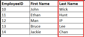
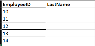
Let’s walk through a real-world scenario. Imagine you have a list of Employee IDs in one column, and you need to pull their Last Names from a master database.
Step 1: Start the Formula
Click the cell where you want the result to appear. Type =VLOOKUP( into the formula bar.
Step 2: Select the “Lookup Value”
Click on the cell that contains the unique identifier you are searching for (e.g., cell A2, which contains the Employee ID). Type a comma.
- Formula so far: =VLOOKUP(A2,
Step 3: Select the “Table Array”
Highlight your master data table. Ensure the column containing the Employee IDs is the first column in your selection.
- Pro Tip: Press F4 on your keyboard immediately after selecting the table. This locks the reference (adding dollar signs like $A$2:$C$100), ensuring the table range doesn’t move if you copy the formula down.
- Formula so far: =VLOOKUP(A2, $A$2:$C$100,
Step 4: Count the Columns
Count columns from left to right within your selected table until you reach the “Last Name” column. If “ID” is column 1 and “Last Name” is column 3, type 3.
- Formula so far: =VLOOKUP(A2, $A$2:$C$100, 3,
Step 5: Choose Exact Match
This is where most beginners make a mistake. You almost always want an Exact Match. Type FALSE or 0.
- Final Formula: =VLOOKUP(A2, $A$2:$C$100, 3, FALSE)
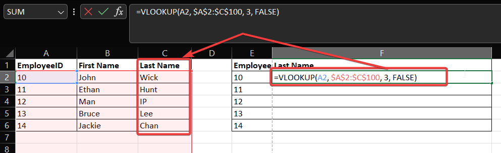
Hit Enter, and the name will appear!
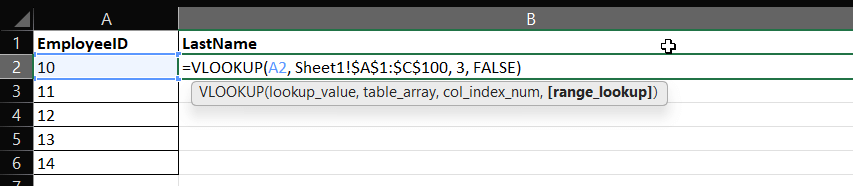
How to apply VLOOKUP from one Excel to another (different sheets or workbooks)?
You don’t need to have your data on the same page. VLOOKUP works perfectly across different sheets (tabs) in your workbook.
The process is identical, but when you select your Table Array, simply click on the other sheet tab and highlight the data there. Excel will automatically add the sheet name to the syntax:
=VLOOKUP(A2, ‘Sheet1’!$A$1:$C$100, 3, FALSE)
Where Sheet1 refer to the master table.
Note the single quotes around the sheet name—Excel adds these automatically if your sheet name has spaces.
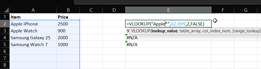
Advanced Tip: VLOOKUP Using Wildcards for Partial Matches
Sometimes you might not know the exact spelling of a lookup value. In these cases, you can use Wildcards:
- Asterisk (*): Matches any sequence of characters.
- Question Mark (?): Matches any single character.
For example, to find the price of an item that starts with “Apple” (like “Apple iPhone” or “Apple Watch”), you can use:
=VLOOKUP(“Apple*”, A2:B99, 2, FALSE)
Pro Trick: VLOOKUP with Multiple Criteria
One of the most common complaints is that VLOOKUP only accepts one lookup value. But what if you need to search for a First Name AND Last Name combined?
Most tutorials skip this, but here is the secret “Helper Column” trick:
- Create a unique key: In your source data, insert a new column to the left. Use the formula =A2&B2 to combine First and Last Name (e.g., “JohnSmith”).
- Combine your lookup value: In your VLOOKUP formula, combine the criteria using the same ampersand (&).
- Formula: =VLOOKUP(H2&I2, A:D, 4, FALSE)
This forces Excel to look for the combined unique identity “JohnSmith” rather than just “John” or “Smith.”
What are some best practices for using VLOOKUP effectively?
Hardcoding numbers like “3” or “4” for the column index is risky—if you insert a new column in your dataset, your VLOOKUP breaks.
To make your formula bulletproof, you can replace the static number with the MATCH function. MATCH finds the column number for you automatically.
- Dynamic Formula: =VLOOKUP(A2, A:E, MATCH(“Price”, A1:E1, 0), FALSE)
In this example, Excel searches for the header “Price” to calculate the column number dynamically. If you move the Price column, the formula updates itself!
The “Dangerous Default” Warning
When learning how to use VLOOKUP in Excel, you must understand its biggest pitfall.
If you leave the last argument (range_lookup) blank, Excel defaults to TRUE (Approximate Match).
This can lead to disastrous results where Excel grabs a “close enough” value if it can’t find the exact one. Unless you are calculating tax brackets or grading scales, always type FALSE.
When to Use Approximate Match (TRUE)
While FALSE is the standard for text and IDs, the Approximate Match (TRUE) is powerful for grouped numbers, such as assigning grades or tax rates.
Example: If you want to assign a grade of “B” to any score between 80 and 89:
- Set up a reference table with scores sorted in ascending order (e.g., 0, 60, 70, 80, 90).
- Use TRUE as the last argument: =VLOOKUP(Score, GradeTable, 2, TRUE).
- Excel will find the largest value that is less than or equal to your lookup value.
Key Requirement: For TRUE to work, the first column of your table must be sorted from smallest to largest, or the formula will return errors.
Troubleshooting Common VLOOKUP Errors
Even the pros get error messages. Here is how to fix the two most common ones:
- #N/A Error: This means “Not Available.” Excel cannot find your lookup value in the first column.
- Check Data Types: A common culprit is “Numbers stored as Text.” If your ID is 123 (number) but the table has 123 (text), VLOOKUP will fail. Use the “Text to Columns” tool to fix this.
- Check Trailing Spaces: “Apple ” is not the same as “Apple”.
- #REF! Error: This means “Reference Invalid.” You likely asked for column number 5, but your selected table only has 4 columns. Adjust your col_index_num.
For a deeper dive into error handling, check out Microsoft’s official support page on VLOOKUP.
Are there any alternatives to VLOOKUP, such as INDEX/MATCH or XLOOKUP?
If you are using Excel 2021 or Microsoft 365, you might be wondering if you should switch to XLOOKUP.
| Feature | VLOOKUP | XLOOKUP |
|---|---|---|
| Direction | Right only | Left or Right |
| Default Match | Approximate (Dangerous) | Exact (Safe) |
| Column Reference | Manual Number (e.g., 3) | Direct Range Selection |
| Insert Columns | Breaks Formula | Auto-updates |
Verdict: Use XLOOKUP for new projects if you have access to it. Continue to use VLOOKUP if you are sharing files with users on older versions of Excel.
Frequently Asked Questions (FAQ)
A: No. VLOOKUP treats “apple”, “APPLE”, and “Apple” as the exact same value.
A: No. VLOOKUP can only search in the first column and return values from columns to the right. To look left, you should use the INDEX and MATCH combo or XLOOKUP.
A: VLOOKUP relies on a static column index number (e.g., “3”). If you insert a column into your table, your data moves to column 4, but the formula still looks at column 3. This is a known limitation of the function.
Conclusion
Mastering this function is a milestone in any data journey. By understanding the four arguments and remembering to lock your cell references, you now know how to use VLOOKUP in Excel to automate tedious searches and reduce manual errors.
Ready to take it to the next level? Open a spreadsheet right now and try looking up a value using FALSE for an exact match. If you found this guide helpful, please share it with your colleagues or leave a comment below with your favorite Excel shortcut!
IT Security / Cyber Security Experts.
Technology Enthusiasm.
Love to read, test and write about IT, Cyber Security and Technology.
The Geek coming from the things I love and how I look.