How to Create a Drop Down List in Excel (Complete Guide)

Struggling with messy, inconsistent data in your spreadsheets? This guide will show you exactly how to create a drop down list in Excel. This powerful tool is your first line of defense against typos and ensures data integrity, making your workbooks cleaner and more professional.

How to Create a Drop Down List in Excel (The 4-Step Method)

First, let’s cover the foundational method. This is the simplest way to get a drop-down list up and running in under a minute.

Step 1: Prepare Your List of Options

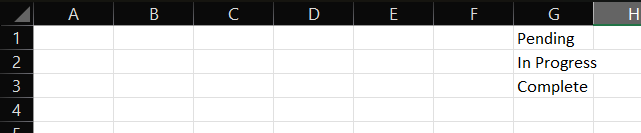
To begin, you need to decide what options will appear in your dropdown. The best practice is to type these items into a single column in your worksheet. For instance, you could place your list of statuses—”Pending,” “In Progress,” and “Complete”—in cells G1:G3.

Pro Tip: It’s a great idea to put this source list on a separate sheet (you could name it “Lists”) to keep your main worksheet tidy.

Step 2: Select the Cell for Your Drop-Down

Next, click on the cell where you want the drop-down arrow to appear. In this case, let’s say it’s cell C2.

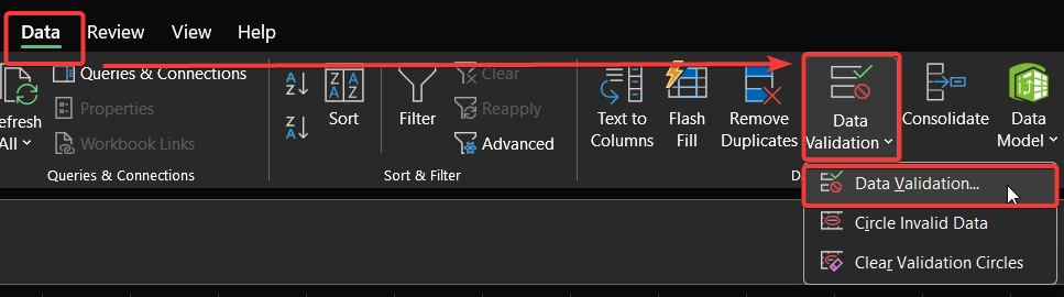
Step 3: Open the Data Validation Tool

With cell C2 selected, navigate to the Data tab on Excel’s top ribbon. In the Data Tools group, you’ll see an icon for Data Validation. Click on it.

Step 4: Configure the List Source

A “Data Validation” dialog box will pop up. This is where the magic happens.

1. Under the Settings tab, click the dropdown under Allow: and select List.
2. An input box labeled Source: will appear. Click inside this box.
3. Now, use your mouse to select the range of cells containing your list (G1:G3).
4. Ensure the In-cell dropdown box is checked.
5. Finally, click OK.

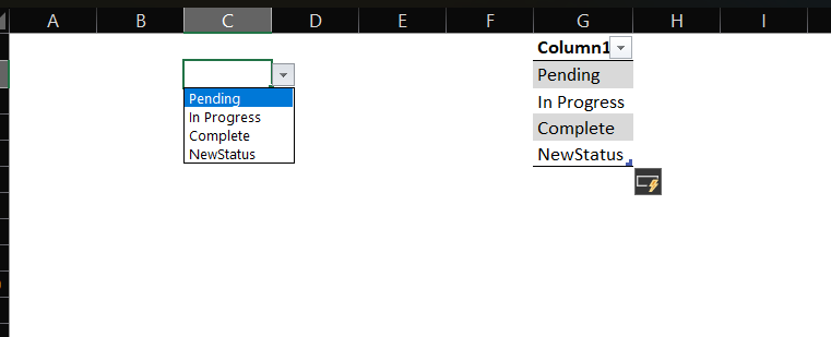
And that’s it! Cell C2 now has a drop-down arrow with your specified options.

The Best Way: How to Create a Drop-Down List from a Dynamic Table

The basic method has one flaw: if you add a new item to your source list, you have to manually update the Data Validation source range. The solution is to use a dynamic Excel Table.

This is the method professionals use because it updates your drop-down list automatically.

1. Select Your Source List: Click any cell within your source list (e.g., G1:G3).
2. Format as Table: Go to the Home tab and click Format as Table. Choose any style you like. In the pop-up, make sure the “My table has headers” box is checked if you have a header, then click OK.
3. Name the Table: Select your new table. A Table Design tab will appear. On the far left, you’ll see a Table Name: box. Give it a simple, memorable name (e.g., StatusList).
4. Update Data Validation: Go back to your drop-down cell (C2), open Data Validation again, and in the Source: box, enter the formula: =INDIRECT(“StatusList”).
5. Click OK.

Now, whenever you add a new item to the bottom of your table, the drop-down list will automatically include it!

Advanced: How to Create a Dependent Drop-Down List

Ever wanted a drop-down list where the options change based on another cell’s value? This is called a dependent (or cascading) drop-down list. For example, selecting a country in one list populates a second list with its corresponding cities.

This technique uses a combination of Named Ranges and the INDIRECT function.

1. Set Up Your Lists: Create your primary list (e.g., “USA,” “Canada” in cells A2:A3). Then, create a separate list for each primary option. The key is that the header for each secondary list must exactly match an item from the primary list.(Image: Screenshot showing one list with “USA” and “Canada,” and two other lists with headers “USA” and “Canada” containing their respective cities.)
2. Create Named Ranges:
   • Select the header and cities for the first secondary list (e.g., “USA” and its cities).
   • Go to the Formulas tab and click Create from Selection.
   • In the pop-up, ensure only Top row is checked and click OK. Excel has now created a Named Range called “USA”.
   • Repeat this process for the “Canada” list.
3. Create the Primary Drop-Down: Use the basic 4-step method to create a drop-down in cell C2 that points to your primary list (A2:A3).
4. Create the Dependent Drop-Down:
   • Select the cell for your dependent list (e.g., D2).
   • Open Data Validation.
   • Choose Allow: List.
   • In the Source: box, enter the formula: =INDIRECT(C2). This tells Excel to look at the value in C2 (e.g., “USA”) and use the Named Range with that same name as the source for this list.
   • Click OK.

Now, when you select “USA” in cell C2, the drop-down in D2 will show American cities. Change C2 to “Canada,” and the D2 options will update instantly.

How to Manage and Customize Your Drop-Down Lists

Creating the list is just the start. Subsequently, you’ll need to manage it.

How to Edit or Delete a Drop-Down List

To edit a list sourced from a cell range, simply change the text in the source cells. If you used the dynamic table method, you can add or remove rows. To completely remove a drop-down, select the cell, open Data Validation, and click the Clear All button.

How to Add Helpful Input Messages and Error Alerts

In the Data Validation window, you have two more useful tabs:

• Input Message: Use this to show a helpful pop-up when a user clicks the cell. For example: “Please select a status from the list.”
• Error Alert: This controls what happens if someone tries to type an invalid entry. You can show a hard Stop that prevents the entry or a softer Warning.

For a deeper dive into these settings, you can review Microsoft’s official documentation on Data Validation.

Frequently Asked Questions (FAQs)

Can I create a drop-down list from a range on another worksheet?

Yes, absolutely! When you are in the Source: box of the Data Validation tool, simply click on the tab for the other worksheet and select the range there. Excel handles the cross-sheet reference automatically.

Why isn’t my drop-down list showing all the items?

This is a common issue when you’re not using the dynamic table method. It usually means you’ve added items to your source list, but you haven’t updated the range in the Data Validation settings. To fix this, select your drop-down cell, go back into Data Validation, and re-select the entire source range, including your new items.

Conclusion: Take Control of Your Data

Congratulations! You are now equipped with a vital Excel skill. By knowing how to create a drop down list in Excel, you can build spreadsheets that are more accurate, efficient, and user-friendly. You’ve learned the basic method, the superior dynamic method, and even the advanced dependent list technique.

The next step is to put this knowledge into practice. Use it in your next report to prevent data entry errors before they happen. If you found this guide helpful, please share it with a colleague! What other Excel challenges are you facing? Let me know in the comments below.

Zachary Allen 'The Geek'

IT Security / Cyber Security Experts.
Technology Enthusiasm.
Love to read, test and write about IT, Cyber Security and Technology.
The Geek coming from the things I love and how I look.