
Learning how to remove duplicates in excel is the first step to transforming a messy, unreliable spreadsheet into a clean, accurate dataset. Duplicate rows can skew your analysis and lead to costly errors, but thankfully, Excel provides several powerful ways to eliminate them with precision and ease.
This guide will walk you through seven distinct methods, from the simple one-click tool for beginners to advanced techniques for experts.
- Key Takeaways
- Before You Begin: A Crucial Best Practice
- Why Removing Duplicates is Critical for Your Data
- How To Remove Duplicates in Excel
- Method 1: The Easiest Way with Excel’s “Remove Duplicates” Tool
- Method 2: Find and Highlight Duplicates with Conditional Formatting
- Method 3: More Control with the Advanced Filter
- Method 4: A Dynamic Solution Using the COUNTIF Formula
- Method 5: The Modern Way with the UNIQUE Function
- Method 6: Automation for Large Datasets with Power Query
- Method 7: Ultimate Customization with a VBA Macro
- Troubleshooting: Why ‘Remove Duplicates’ Might Not Be Working
- Comparison: Which Method is Right for You?
- Frequently Asked Questions (FAQ)
- Conclusion: Master Your Data Today
Key Takeaways
- Safety First: Always work on a copy of your data, as the main “Remove Duplicates” tool permanently deletes rows.
- The Quickest Fix: For a fast, permanent cleanup, the go-to solution is the Remove Duplicates button located on the Data tab. (Click here for details)
- Find, Don’t Delete: Use Conditional Formatting from the Home tab when you only want to highlight and review duplicates without removing them.
- Advanced & Dynamic Solutions: For more control, use Formulas (like UNIQUE), Power Query, or the Advanced Filter to create separate, non-destructive lists of unique values.
- Troubleshoot Invisible Errors: If duplicates aren’t found, it’s likely due to hidden spaces or numbers stored as text. Use the TRIM and CLEAN functions to fix your data first.
Before You Begin: A Crucial Best Practice
Always work on a copy of your data. Methods like the built-in “Remove Duplicates” tool permanently delete rows from your dataset. To avoid irreversible mistakes, it’s highly recommended that you either duplicate your worksheet or save a new version of the file before you start cleaning your data.
Why Removing Duplicates is Critical for Your Data
Before we dive into the “how,” let’s quickly cover the “why.” Duplicate data undermines data integrity. It can lead to inaccurate counts, skewed averages, and flawed reports.
Consequently, cleaning your dataset by removing these redundant entries is a fundamental step in any data analysis process, ensuring your conclusions are based on reliable information.
Pro Tip: Convert Your Data to an Excel Table First
For a more robust and professional workflow, convert your data range into a formal Excel Table before applying any of these methods. Simply click anywhere in your data and press Ctrl + T.
Benefits of using a Table:
- Auto-Expanding Ranges: When you add new rows or columns, they are automatically included in the table, so your duplicate-removal logic doesn’t miss new data.
- Easy Formatting: Tables come with built-in styling for enhanced readability.
- Structured Referencing: Formulas become easier to read and manage.
How To Remove Duplicates in Excel
Method 1: The Easiest Way with Excel’s “Remove Duplicates” Tool
This is the go-to method for most users. It’s fast, straightforward, and built directly into Excel.
When to Use This Method
This approach is ideal for a quick, permanent cleanup of your data. It works by deleting the entire row of any subsequent duplicate entry it finds, keeping only the first unique instance.
Step-by-Step Instructions
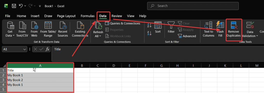
- Select Your Data: First, click any cell within your data range. Excel is smart enough to detect the entire table automatically.
- Navigate to the Data Tab: Next, go to the Data tab on the Excel ribbon.
- Click Remove Duplicates: In the Data Tools group, click the Remove Duplicates button.
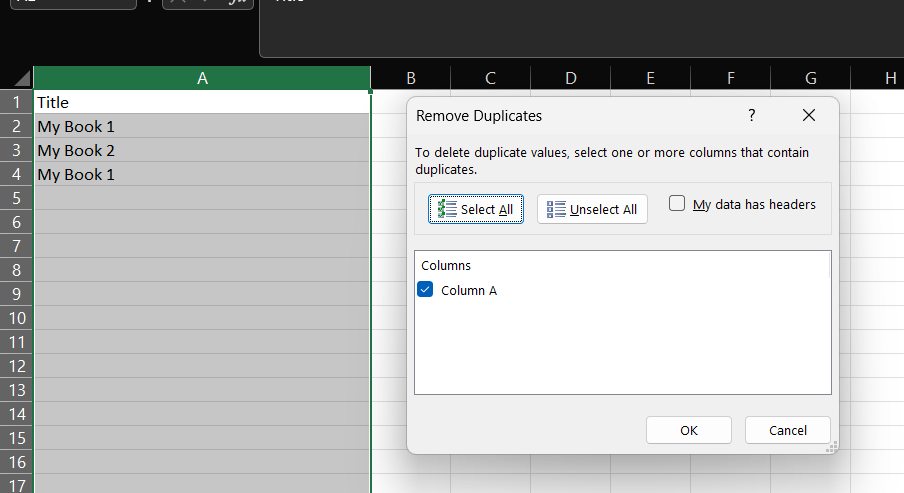
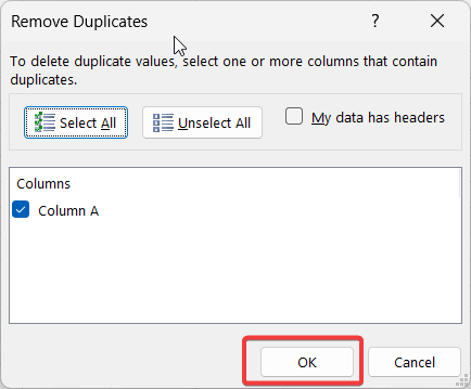
- Configure Columns: A dialog box will appear. If your data has headers, ensure “My data has headers” is checked. Then, select the columns you want Excel to check for duplicate values. To find rows that are exact copies, leave all columns checked.
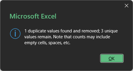
- Execute and Review: Finally, click OK. Excel will immediately delete the duplicate rows and show a message telling you how many duplicates were removed and how many unique values remain.
Pros & Cons
- Pro: Extremely fast and user-friendly.
- Con: It’s a destructive action; the data is permanently deleted. Therefore, it’s wise to work on a copy of your file.
Read more article related to Microsoft Excel.
Method 2: Find and Highlight Duplicates with Conditional Formatting
What if you want to find the duplicates without deleting them right away? Conditional Formatting is your best friend.
When to Use This Method
Use this non-destructive method when you need to review duplicate entries before deciding what to do with them.
Step-by-Step Instructions
- Select the Column: First, highlight the column where you want to check for duplicates.
- Open Conditional Formatting: On the Home tab, click Conditional Formatting, then go to Highlight Cells Rules, and select Duplicate Values.
- Choose Formatting: In the dialog box, you can choose how you want the duplicates to be formatted (e.g., “Light Red Fill with Dark Red Text”). Then, click OK.
- Review: All duplicate values in your selected column will now be highlighted, making them easy to spot.
Pros & Cons
- Pro: Non-destructive and visual. Allows for manual review.
- Con: Doesn’t remove anything; it’s purely for identification.
Method 3: More Control with the Advanced Filter
The Advanced Filter is another powerful tool that can help you extract a list of unique values, leaving your original data completely untouched.
When to Use This Method
This is perfect when you need to create a new, clean list of unique records in a different location in your worksheet.
Step-by-Step Instructions
- Select Your Data: First, click a cell inside your dataset.
- Open Advanced Filter: Go to the Data tab and click Advanced in the Sort & Filter group.
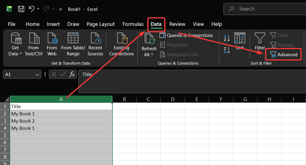
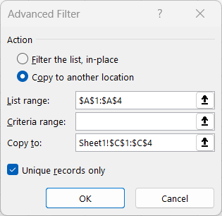
- Configure the Filter: In the dialog box, select Copy to another location. The List range should already be your data. Click in the Copy to box and select the cell where you want your new, unique list to start. Most importantly, check the box for Unique records only.
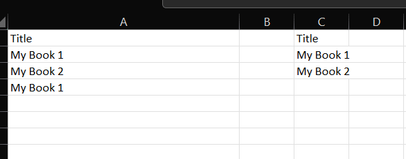
- Click OK: Excel will immediately create a new list of unique values in the location you specified.
Pros & Cons
- Pro: Non-destructive and creates a separate, clean list.
- Con: Slightly more complex than the main “Remove Duplicates” tool.
Method 4: A Dynamic Solution Using the COUNTIF Formula
For a more dynamic approach, you can use a formula to flag duplicates. This is great for data that is updated frequently.
When to Use This Method
Use a formula when you need a real-time indicator of duplicates as new data is entered.
Step-by-Step Instructions
- Create a Helper Column: First, add a new column next to your data and label it something like “IsDuplicate?”
- Enter the COUNTIF Formula: In the first cell of your new column (e.g., C2), enter the following formula: =IF(COUNTIF($B$2:$B$10, B2)>1, “Duplicate”, “Unique”)
- $B$2:$B$10 is the absolute range of cells you want to check.
- B2 is the cell in the current row you’re checking.
(Image: Screenshot showing the COUNTIF formula entered into the helper column.)
- Drag the Formula Down: Finally, click the small square in the bottom-right corner of the cell and drag it down to apply the formula to all rows. The formula will now flag each row as either “Duplicate” or “Unique.”
Pros & Cons
- Pro: Dynamic and updates automatically. Non-destructive.
- Con: Requires a helper column and knowledge of formulas.
Method 5: The Modern Way with the UNIQUE Function
If you have a modern version of Excel (Microsoft 365 or Excel 2021), the UNIQUE function is a game-changer. It dynamically creates a list of unique values in a single step.
When to Use This Method
Use this when you want the simplest, fastest, and most modern way to generate a list of unique values from a range or column.
Step-by-Step Instructions
- Select a Destination Cell: Click an empty cell where you want your list of unique values to begin.
- Enter the UNIQUE Formula: Type =UNIQUE( and then select the entire range of cells you want to pull unique values from (e.g., A2:A20).
- Close the Formula and Press Enter: Your final formula will look something like this: =UNIQUE(A2:A20). Press Enter.
(Image: Screenshot showing the UNIQUE formula and the resulting dynamic array of unique values.) - Review the Output: Excel will instantly spill the unique values into the cells below your formula. This list will automatically update if the source data changes.
Pros & Cons
- Pro: Incredibly simple and powerful. The resulting list is dynamic.
- Con: Only available in modern versions of Excel.
Method 6: Automation for Large Datasets with Power Query
For the ultimate in power and automation, especially with large datasets, look no further than Power Query.
When to Use This Method
Power Query is the best tool when you are dealing with very large files, need to pull data from external sources, or want to create a repeatable, automated process for cleaning your data.
Step-by-Step Instructions
- Load Data into Power Query: Select your data range, go to the Data tab, and click From Table/Range.
- Use Remove Duplicates: The Power Query Editor will open. Right-click the header of the column you want to check for duplicates. In the context menu, select Remove Duplicates.
(Image: Screenshot of the Power Query editor with the “Remove Duplicates” option.) - Close & Load: Finally, click Close & Load in the top-left corner. Power Query will create a new sheet in your workbook with a clean, de-duplicated table. The best part? You can simply hit “Refresh” to re-run the process anytime your source data changes. For more information, you can explore the official Microsoft Power Query documentation.
Pros & Cons
- Pro: Extremely powerful, automatable, and handles huge datasets efficiently.
- Con: Has a steeper learning curve for new users.
Method 7: Ultimate Customization with a VBA Macro
For complete control and automation, you can use a Visual Basic for Applications (VBA) macro. This is an advanced technique but offers maximum flexibility.
When to Use This Method
Use a VBA macro when you need to perform a duplicate removal task repeatedly as part of a larger automated workflow.
Step-by-Step Instructions
- Open the VBA Editor: Press Alt + F11 to open the VBA editor.
- Insert a New Module: In the editor, go to Insert > Module.
- Paste the Code: Copy and paste the following code into the module window:codeVba
Sub RemoveDuplicatesMacro() ' This macro removes duplicate rows based on the entire row's content ' from the active worksheet. Dim ws As Worksheet Set ws = ActiveSheet ws.Range("A1").CurrentRegion.RemoveDuplicates Columns:=Array(1, 2, 3), Header:=xlYes ' Note: Change Array(1,2,3) to the columns you want to check End Sub - Run the Macro: Close the editor, press Alt + F8, select RemoveDuplicatesMacro from the list, and click Run.
Pros & Cons
- Pro: Fully automatable and customizable for complex tasks.
- Con: Requires macros to be enabled, which can be a security concern. Intimidating for beginners.
Troubleshooting: Why ‘Remove Duplicates’ Might Not Be Working
Have you ever used the “Remove Duplicates” tool, only for it to find zero duplicates when you can clearly see them? This common frustration is usually caused by “invisible” data issues. Here’s how to fix them.
Problem 1: Hidden Trailing or Leading Spaces
Excel sees “Apple ” (with a space at the end) and “Apple” as two completely different values.
- Solution: Use the TRIM function. Create a helper column and use the formula =TRIM(A2) (where A2 is the cell with your text). This will remove all extra spaces. Then, copy this new, clean column and paste it back over the original as values.
Problem 2: Numbers Stored as Text
Sometimes, a number like 12345 can be formatted as text. Excel will not see it as a duplicate of the actual number 12345.
- Solution: Look for the small green triangle in the corner of the cell. Click it, and choose Convert to Number. This will reformat the text back into a true number that Excel can correctly compare.
Problem 3: Non-Printing Characters
Data copied from websites can contain hidden characters like line breaks.
- Solution: Use the CLEAN function. Similar to TRIM, use the formula =CLEAN(A2) in a helper column to remove these non-printing characters. Copy and paste the cleaned data as values over your original column.
Comparison: Which Method is Right for You?
| Method | Best For | Speed | Destructive? | Complexity |
|---|---|---|---|---|
| Remove Duplicates Tool | Quick, one-time cleanups | Very Fast | Yes | Low |
| Conditional Formatting | Visually identifying duplicates | Fast | No | Low |
| Advanced Filter | Creating a separate unique list | Fast | No | Medium |
| COUNTIF Formula | Dynamic, real-time checking | Medium | No | Medium |
| UNIQUE Function | Modern, dynamic unique lists | Very Fast | No | Low |
| Power Query | Large datasets & automation | Fast | No | High |
| VBA Macro | Custom, repeatable workflows | Very Fast | Yes | Very High |
Frequently Asked Questions (FAQ)
Q1: How do I remove duplicates in Excel but keep the first one?
This is the default behavior of the main Remove Duplicates tool (Method 1). It automatically scans from top to bottom and keeps the very first instance of a record it finds, deleting all subsequent matches.
Q2: How do I remove duplicates but keep the last instance instead?
This is a great question that requires a clever two-step process. First, sort your data in reverse order (Z to A, or largest to smallest). Then, use the standard Remove Duplicates tool. Because the tool keeps the first item it sees, and you’ve reversed the list, it will be keeping what was originally the last instance.
Q3: Can I remove duplicates based on only one column?
Absolutely. In the “Remove Duplicates” dialog box (Method 1), you can uncheck all columns except for the single column you want to use as the basis for finding duplicates. Excel will then delete any row where the value in that specific column is a duplicate.
Q4: How do I handle case-sensitive duplicates (e.g., treat “apple” and “Apple” as different)?
The standard “Remove Duplicates” tool is not case-sensitive. For a case-sensitive removal, you would need to use a more advanced approach, typically with a formula involving the EXACT function or by using Power Query, which has case-sensitive options.
Conclusion: Master Your Data Today
Now that you know how to remove duplicates in excel, you’re equipped with a full toolkit to handle any scenario. From the instant fix of the Remove Duplicates tool to the automated power of Power Query and VBA, you can ensure your spreadsheets are clean, accurate, and reliable. Choose the method that best fits your task, and you’ll save time and gain confidence in your data. To help you master these techniques, consider creating a practice workbook with the examples in this guide.
Which method will you try first? Share your experience in the comments below
IT Security / Cyber Security Experts.
Technology Enthusiasm.
Love to read, test and write about IT, Cyber Security and Technology.
The Geek coming from the things I love and how I look.